#This is a comment

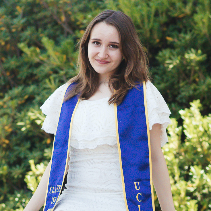
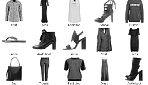
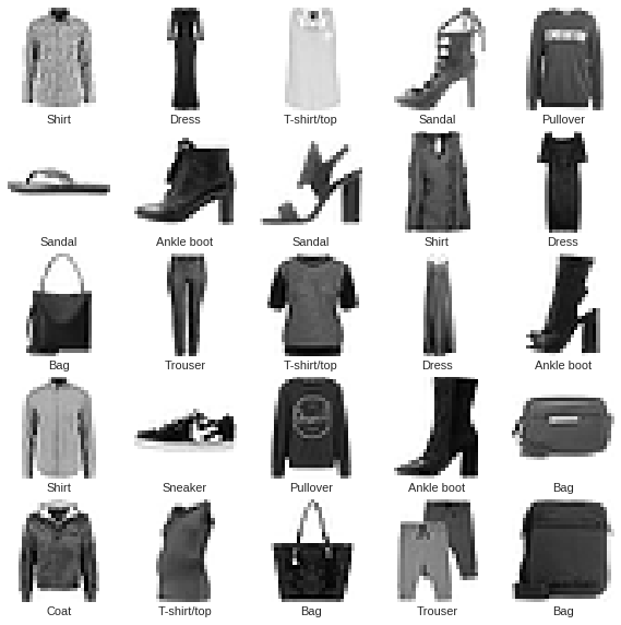
Fashion-MNIST samples (by Zalando, MIT License).

Training and Testing

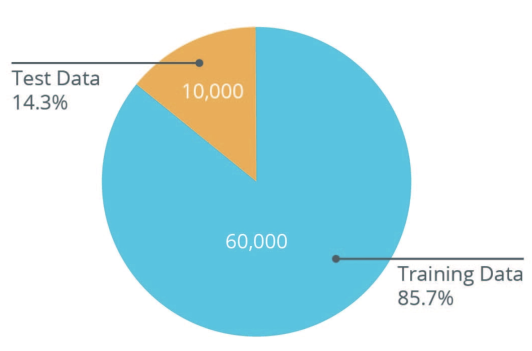Most of the images will be used as training data to tune the model. However, 10,000 images will be set aside to see how the model performs on images it has never seen before. This decreases chances of overfitting the model.

It is common to use what is called a Validation dataset. This dataset is not used for training. Instead, it it used to test the model during training. This is done after some set number of training steps, and gives us an indication of how the training is progressing. For example, if the loss is being reduced during training, but accuracy deteriorates on the validation set, that is an indication that the model is simply memorizing the training set.

Model Layers

Because each image is 28×28 pixels, there needs to be 784 nodes (the total area) in the input layer. This is because the 2D image is converted into a one-dimensional array. This process is called flattening. In code, this is done with a flatting layer.

tf.keras.layers.Flatten (input_shape=(28, 28, 1))

Then there is a dense layer, which has 128 units in this example. ReLU (Rectified Linear Unit) gives the dense layer more power. ReLU is a type of activation function that allows to solve for nonlinear problems. Last time we had a y=mx+b format for the Celsius to Fahrenheit conversion, but most problems won’t be linear. There several of these functions (ReLU, Sigmoid, tanh, ELU), but ReLU is used most commonly and serves as a good default. f(x) = max(0, x)

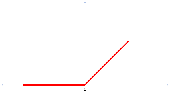
tf.keras.layers.Dense(128, activation=tf.nn.relu)

The output layer contains 10 units, because the fashion MNIST datasets contains 10 labels for clothing. Each unit specifies the probability that the inputted image of clothing belongs to that label. For example if you input an image of a t-shirt, it may be outputted as .88 t-shit (label=0), .04 trouser (label = 1), .1 pullover (label = 2), etc. This is how confident the model is that the image belongs to each clothing group. The goal is to get the percentage for t-shit as high as possible after training the model so that the image is classified correctly. The actual percentages should be 1 t-shirt (label = 0), 0 trouser (label=1), 0 pullover (label = 2), etc.

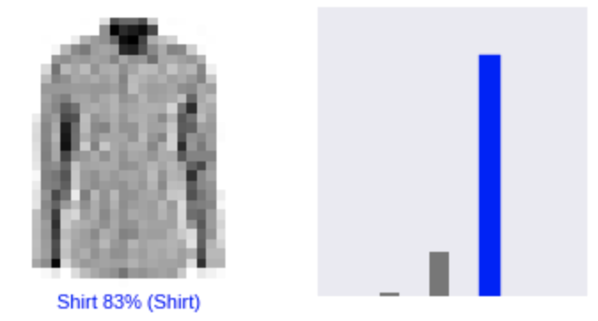
Here is an example of what might be outputted with an image of a shirt:

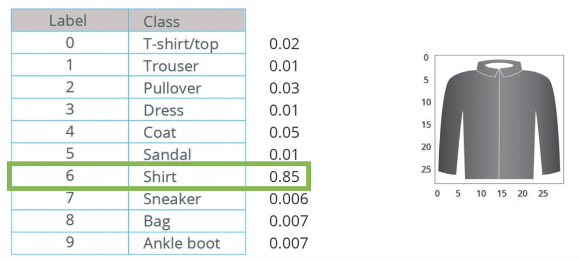The model is 85% confident this image is of a shirt. Notice the percentages sum to 1. This is a probability distribution.

tf.keras.layers.Dense(10, activation=tf.nn.softmax)

Softmax: A function that provides probabilities for each possible output class.

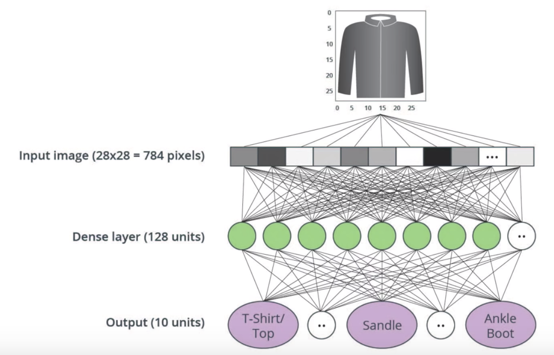A visual of each layer of the neural network.

Classifying Images of Clothing

1. Install and import dependencies

MNIST fashion dataset is in tensorflow_datasets so we can install these.

!pip install -U tensorflow_datasets

Now import tensorflow and some libraries needed.

from __future__ import absolute_import, division, print_function
# Import TensorFlow and TensorFlow Datasets
import tensorflow as tf
import tensorflow_datasets as tfds
tf.logging.set_verbosity(tf.logging.ERROR) 
 
# Helper libraries
import math
import numpy as np
import matplotlib.pyplot as plt 
 
# Improve progress bar display
import tqdm
import tqdm.auto tqdm.tqdm = tqdm.auto.tqdm 
 
print(tf.__version__)
 
# This will go away in the future.
# If this gives an error, you might be running TensorFlow 2
# or above
# If so, the just comment out this line and run this
# cell again
tf.enable_eager_execution()

The MNIST data can be accessed via the dataset API. It then should be split into the training and testing data. Class names aren’t included so you can create a vector of them.

dataset, metadata = tfds.load('fashion_mnist',
as_supervised=True, with_info=True)
 
train_dataset, test_dataset = dataset['train'], dataset['test']
 
class_names = ['T-shirt/top','Trouser','Pullover','Dress','Coat',
               'Sandal','Shirt','Sneaker','Bag','Ankle boot']

*Explore the Data

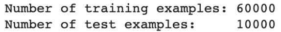
num_train_examples = metadata.splits['train'].num_examples
num_test_examples = metadata.splits['test'].num_examples
print("Number of training examples: {}".format(num_train_examples))
print("Number of test examples: {}".format(num_test_examples))

2. Preprocess the data

The value of each pixel in the image data is an integer in the range [0,255]. This is because the 28×28 images have pixel values ranging from 0 to 255. For the model to work properly, these values need to be normalized to the range [0,1]. So here we create a normalization function, and then apply it to each image in the test and train datasets.

def normalize(images, labels):
  images = tf.cast(images, tf.float32)
  images /= 255
  return images, labels 
 
# The map function applies the normalize function to each
# element in the train and test datasets 
 
train_dataset = train_dataset.map(normalize)
test_dataset = test_dataset.map(normalize)

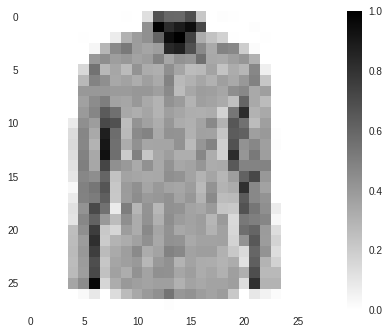
*Explore the processed data

Let’s take a look at an image! Notice the color scale is from 0 to 1 (instead of 0 to 255).

# Take a single image, and remove the color dimension by reshaping
for image, label in test_dataset.take(1):
  break
image = image.numpy().reshape((28,28)) 
 
# Plot the image - voila a piece of fashion clothing
plt.figure()
plt.imshow(image, cmap=plt.cm.binary)
plt.colorbar()
plt.grid(False)
plt.show()

Display the first 25 images from the training set and display the class name below each image. Verify that the data is in the correct format and we’re ready to build and train the network.

plt.figure(figsize=(10,10))
i = 0
for (image, label) in test_dataset.take(25):
  image = image.numpy().reshape((28,28))
  plt.subplot(5,5,i+1)
  plt.xticks([])
  plt.yticks([])
  plt.grid(False)
  plt.imshow(image, cmap=plt.cm.binary)
  plt.xlabel(class_names[label])
  i += 1
plt.show()

3. Build the model

To build the neural network we need to first configure the layers of the model then compile the model.

* Setup the layers

The basic building block of a neural network is the layer. Earlier we discussed the input, dense, and output layer. Much of deep learning consists of chaining together simple layers. Most layers, like tf.keras.layers.Dense, have internal parameters which are adjusted (“learned”) during training.

model = tf.keras.Sequential([
    tf.keras.layers.Flatten(input_shape=(28, 28, 1)),
    tf.keras.layers.Dense(128, activation=tf.nn.relu),
    tf.keras.layers.Dense(10,  activation=tf.nn.softmax)
])

To recap, this neural network has three following layers:

• input tf.keras.layers.Flatten — This layer transforms the images from a 2d-array of 28 × 28 pixels), to a 1d-array of 784 pixels (28*28). Think of this layer as unstacking rows of pixels in the image and lining them up. This layer has no parameters to learn, as it only reformats the data.
• hidden tf.keras.layers.Dense— A densely connected layer of 128 neurons. Each neuron (or node) takes input from all 784 nodes in the previous layer, weighting that input according to hidden parameters which will be learned during training, and outputs a single value to the next layer.
• output tf.keras.layers.Dense — A 10-node softmax layer, with each node representing a class of clothing. As in the previous layer, each node takes input from the 128 nodes in the layer before it. Each node weights the input according to learned parameters, and then outputs a value in the range [0, 1], representing the probability that the image belongs to that class. The sum of all 10 node values is 1.

* Compile the model

Before the model is ready for training, we add a few settings to the compile step:

• Loss function — An algorithm for measuring how far the model’s outputs are from the desired output. We want to minimize the losses. The conventional way is to have the target outputs converted to the one-hot encoded array to match with the output shape, but with sparse_categorical_crossentropy, we can keep the integers as targets.
• Optimizer —An algorithm for adjusting the inner parameters of the model in order to minimize loss.

Adam is an optimization algorithm that can used instead of the classical stochastic gradient descent procedure to update network weights iterative based in training data.

Adam: A Method for Stochastic Optimization, 2015.

• Metrics —Used to monitor the training and testing steps. The following example uses accuracy, the fraction of the images that are correctly classified.

optimizer = tf.train.AdamOptimizer(learning_rate=1e-4,
beta1=0.99, epsilon=0.1)
model.compile(optimizer, loss='sparse_categorical_crossentropy',
metrics=['accuracy'])

4. Train the model

First, we define the iteration behavior for the train dataset:

1. Repeat forever by specifying dataset.repeat() (the epochs parameter described below limits how long we perform training).
2. The dataset.shuffle(60000) randomizes the order so our model cannot learn anything from the order of the examples.
3. And dataset.batch(32) tells model.fit to use batches of 32 images and labels when updating the model variables.

Training is performed by calling the model.fit method:

1. Feed the training data to the model using train_dataset.
2. The model learns to associate images and labels.
3. The epochs=5 parameter limits training to 5 full iterations of the training dataset, so a total of 5 * 60,000 = 300,000 examples.

BATCH_SIZE = 32
train_dataset = train_dataset.repeat().
  shuffle(num_train_examples).batch(BATCH_SIZE)
test_dataset = test_dataset.batch(BATCH_SIZE)
 
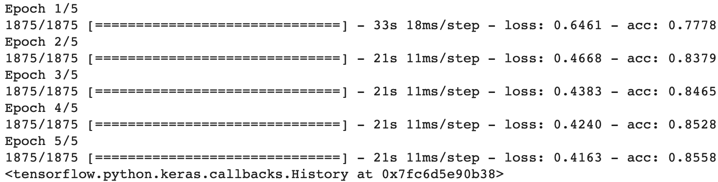
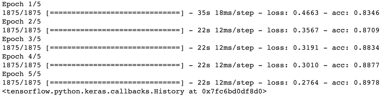
model.fit(train_dataset, epochs=5,
  steps_per_epoch=math.ceil(num_train_examples/BATCH_SIZE))

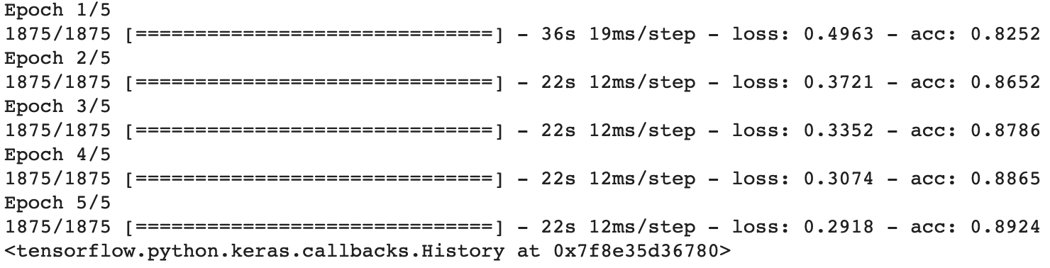
As the model trains, the loss and accuracy metrics are displayed. This model reaches an accuracy of about 89% on the training data.

5. Evaluate the model

The model classifies training images with 89% accuracy, but how does it perform on images it has never seen before? We want to make sure the model didn’t just memorize the training images.

test_loss, test_accuracy = model.evaluate(test_dataset,
  steps=math.ceil(num_test_examples/32)) 
 
print('Accuracy on test dataset:', test_accuracy)

It is less accurate with the test data, but that is expected since the model was trained on the train_dataset.

6. Make predictions and explore

With the model trained, we can use it to make predictions about some images.

for test_images, test_labels in test_dataset.take(1):
  test_images = test_images.numpy()
  test_labels = test_labels.numpy()
  predictions = model.predict(test_images)
 
predictions.shape

32 images with 10 label (clothing group) predictions.

predictions[0]

Which is the highest? Check the test label to see if this is correct.

np.argmax(predictions[0])
 
test_labels[0]

Both of the outputs are 6.

def plot_image(i, predictions_array, true_labels, images):
  predictions_array, true_label, img = predictions_array[i],
  true_labels[i], images[i]
  plt.grid(False)
  plt.xticks([])
  plt.yticks([]) 
 
  plt.imshow(img[...,0], cmap=plt.cm.binary) 
 
  predicted_label = np.argmax(predictions_array)
  if predicted_label == true_label: color = 'blue'
  else: color = 'red'
  plt.xlabel("{} {:2.0f}% ({})".format(class_names[predicted_label],
                                100*np.max(predictions_array),
                                class_names[true_label]),
                                color=color)
 
def plot_value_array(i, predictions_array, true_label):
  predictions_array, true_label = predictions_array[i],true_label[i]
  plt.grid(False)
  plt.xticks([])
  plt.yticks([])
  thisplot = plt.bar(range(10), predictions_array, color="#777777")
  plt.ylim([0, 1])
  predicted_label = np.argmax(predictions_array)
  thisplot[predicted_label].set_color('red')
  thisplot[true_label].set_color('blue')

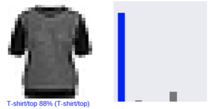
Let’s look at the 0th image, predictions, and prediction array. Correct prediction labels are blue and incorrect prediction labels are red.

i = 0
plt.figure(figsize=(6,3))
plt.subplot(1,2,1)
plot_image(i, predictions, test_labels, test_images)
plt.subplot(1,2,2)
plot_value_array(i, predictions,  test_labels)

i = 12
plt.figure(figsize=(6,3))
plt.subplot(1,2,1)
plot_image(i, predictions, test_labels, test_images)
plt.subplot(1,2,2)
plot_value_array(i, predictions,  test_labels)

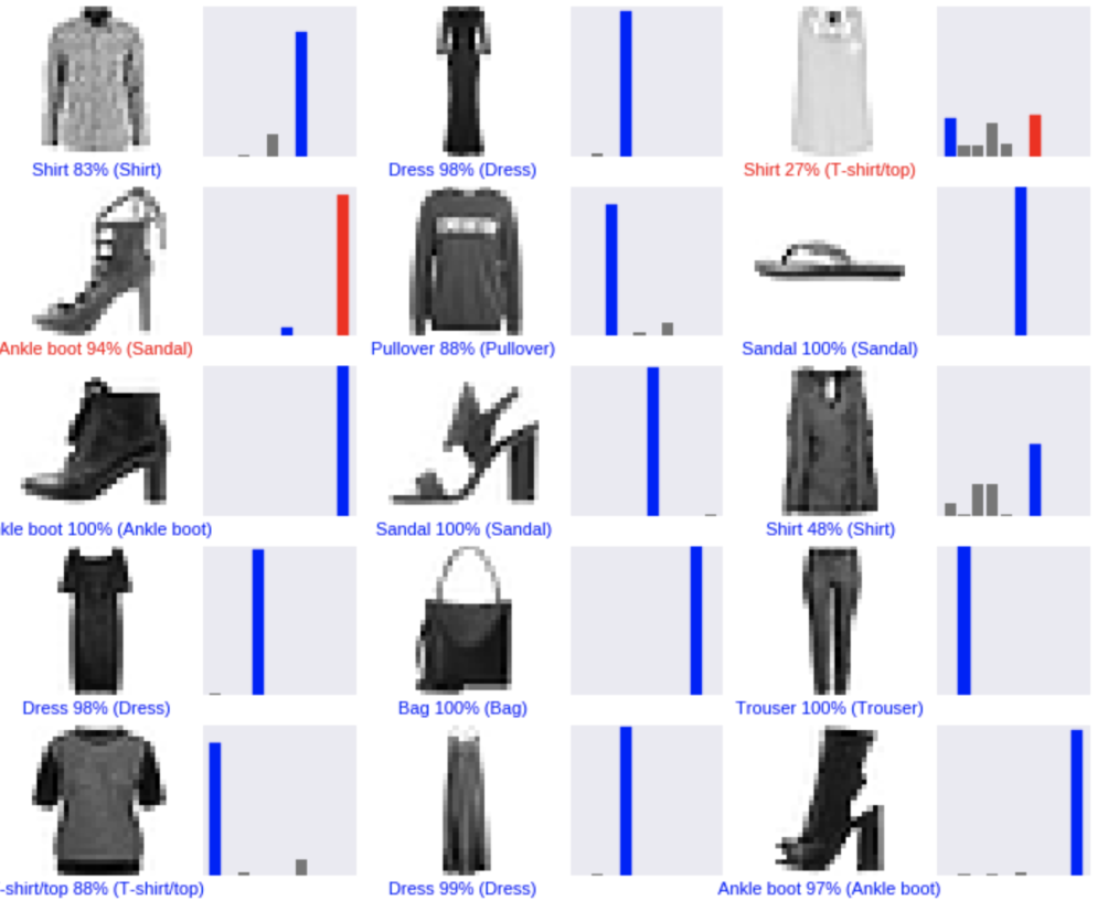
Let’s plot several images with their predictions. Note that even when the model is very confident, it is not necessarily correct.

# Plot the first X test images, their predicted label,
# and the true label
# Color correct predictions in blue, incorrect predictions in red
num_rows = 5
num_cols = 3
num_images = num_rows*num_cols
plt.figure(figsize=(2*2*num_cols, 2*num_rows))
for i in range(num_images):
  plt.subplot(num_rows, 2*num_cols, 2*i+1)
  plot_image(i, predictions, test_labels, test_images)
  plt.subplot(num_rows, 2*num_cols, 2*i+2)
  plot_value_array(i, predictions, test_labels)

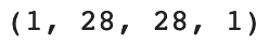
Finally, use the trained model to make a prediction about a single image.

# Grab an image from the test dataset
img = test_images[0]
print(img.shape)

tf.keras models are optimized to make predictions on a batch, or collection, of examples at once. So even though we’re using a single image, we need to add it to a list:

# Add the image to a batch where it's the only member.
img = np.array([img])
print(img.shape)

predictions_single = model.predict(img)
print(predictions_single)

plot_value_array(0, predictions_single, test_labels)
_ = plt.xticks(range(10), class_names, rotation=45)
 
np.argmax(predictions_single[0])

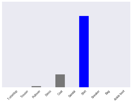
The model predicted 6, a shirt.

7. Exercises

• Set training epochs set to 1 With 1 epoch instead of 5 the accuracy lowers from 89% to 82.6%. This is because the epochs parameter limits how long we perform training.

• Number of neurons in the Dense layer following the Flatten one. For example, go really low (e.g. 10) in ranges up to 512 and see how accuracy changes

With 10 neurons in the Dense layer, the accuracy decreases from 89% to 85.5%.

With 512 neurons in the Dense layer, the accuracy increased from 89.24% to 89.78%

• Add additional Dense layers between the Flatten and the final Dense(10, activation=tf.nn.softmax), experiment with different units in these layers. The original test accuracy was 87.4%. Adding an additional Dense layer with 158 nodes increased the test data accuracy to 88.1%. Adding a Dense layer with 10 nodes slightly decreased the test accuracy to 87.3%. Adding a Dense layer with 512 nodes increased the training accuracy to 89.7% but slightly decreased the test accuracy to 87.3%. This could be a sign of overfitting.