Material follows a Udacity Tensorflow course.

Artificial Intelligence

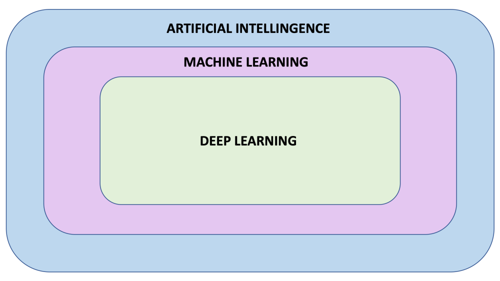
A field of computer science that aims to make computers achieve human-style intelligence. There are many approaches to reaching this goal, including machine learning and deep learning.

• Machine Learning
  A set of related techniques in which computers are trained to perform a particular task rather than by explicitly programming them.
• Neural Network
  A construct in Machine Learning inspired by the network of neurons (nerve cells) in the biological brain. Neural networks are a fundamental part of deep learning, and will be covered in this course.
• Deep Learning
  A subfield of machine learning that uses multi-layered neural networks. Often, “machine learning” and “deep learning” are used interchangeably.

The three main branches of machine learning are:

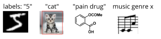
• Supervised Learning
  Using a labeled training dataset to train the computer to make predictions.

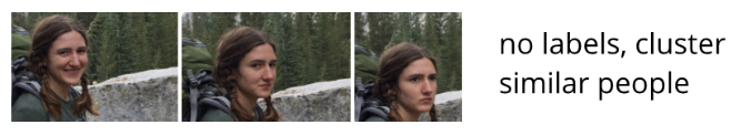
• Unsupervised Learning
  The information used to train is neither classified nor labeled.

• Reinforcement Learning
  An interactive learning method that optimizes a reward.

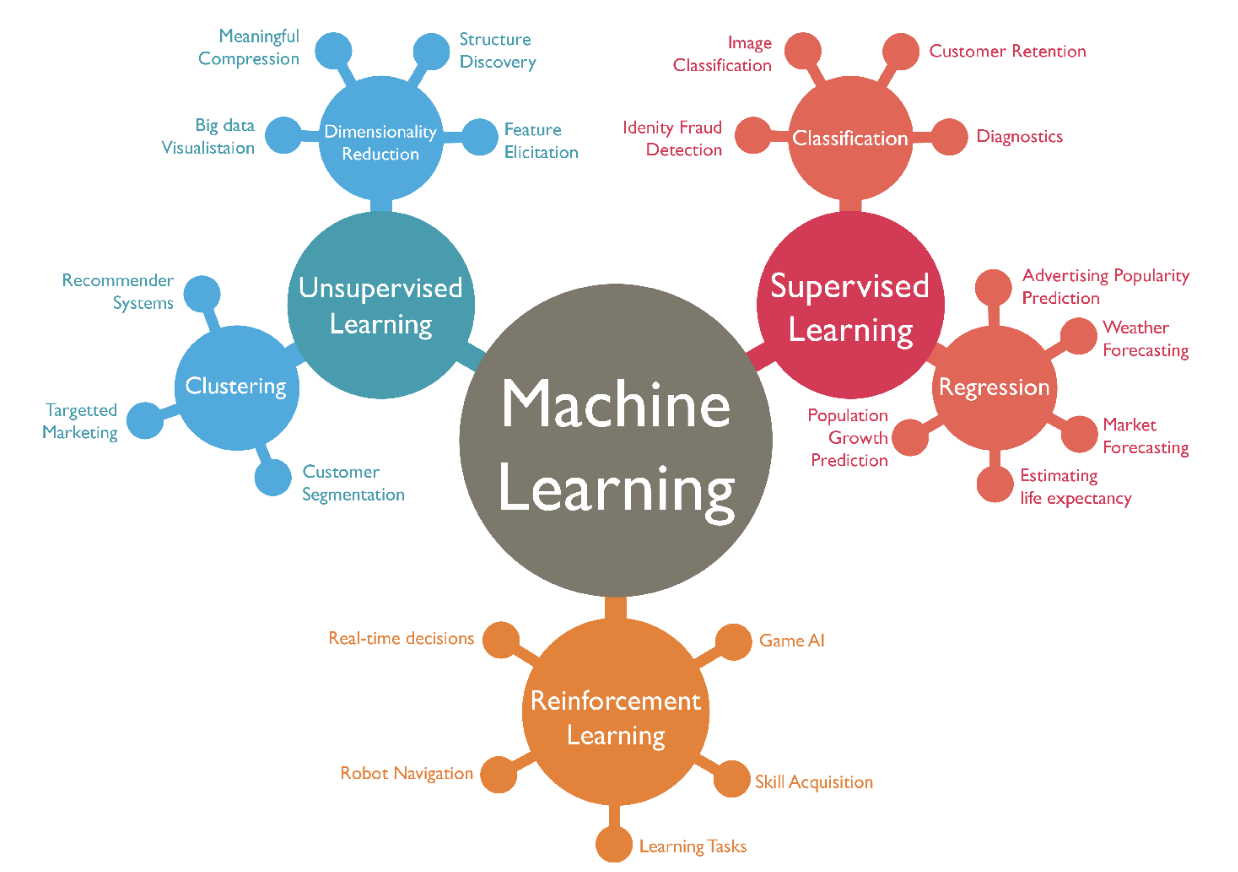
A good visual of the machine learning branches.

Training a First Model in Python

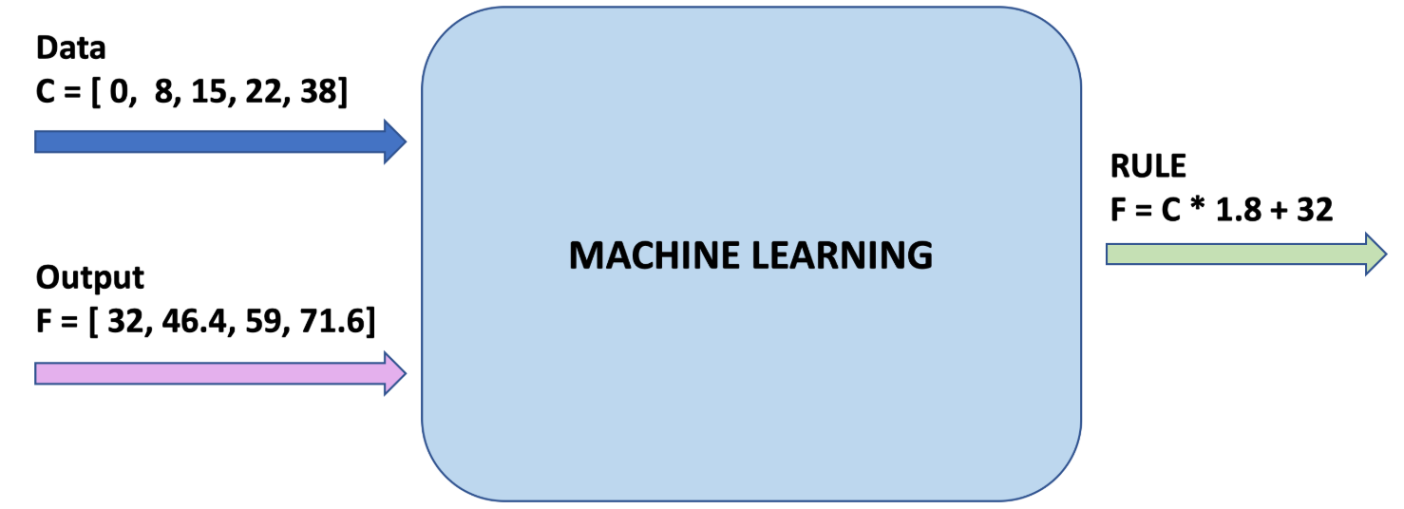
We will use supervised machine learning to find the pattern between Celsius and Fahrenheit values. The formula is 𝑓 = 𝑐 × 1.8 + 32. We will give TensorFlow some sample Celsius values (0, 8, 15, 22, 38) and their corresponding Fahrenheit values (32, 46, 59, 72, 100). Then, we will train a model that figures out the above formula through the training process.

1. Import dependencies

The __future__ statement is intended to ease migration to future versions of Python that introduce incompatible changes to the language. TensorFlow is imported as tf. It will only display errors. Numpy is imported as np. Numpy helps us to represent our data as highly performant lists.

from __future__ import absolute_import, division, print_function
import tensorflow as tf
tf.logging.set_verbosity(tf.logging.ERROR)
 
import numpy as np

2. Set up training data

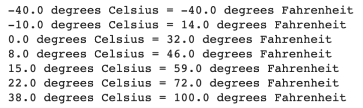
The goal of the model is to provide degrees in Fahrenheit when given degrees in Celsius. So for supervised learning, we give a set of inputs (celsius_q) and a set of outputs (fahrenheit_a) so that the computer can find an algorithm.

celsius_q = np.array([-40, -10, 0, 8, 15, 22, 38],dtype=float)
fahrenheit_a = np.array([-40, 14, 32, 46, 59, 72, 100],dtype=float) 
 
for i,c in enumerate(celsius_q):
    print("{} degrees Celsius = {} degrees Fahrenheit".format(c,
    fahrenheit_a[i]))

• Some Machine Learning terminology:
  Feature — The input(s) to our model. In this case, the degrees in Celsius.
  Labels — The output our model predicts. In this case, the degrees in Fahrenheit.
  Example — A pair of inputs/outputs used during training. In our case a pair of values from celsius_q and fahrenheit_a at a specific index, such as (22,72).

3. Create the model

We will use a Dense network model with only one layer.

• BUILD A LAYER

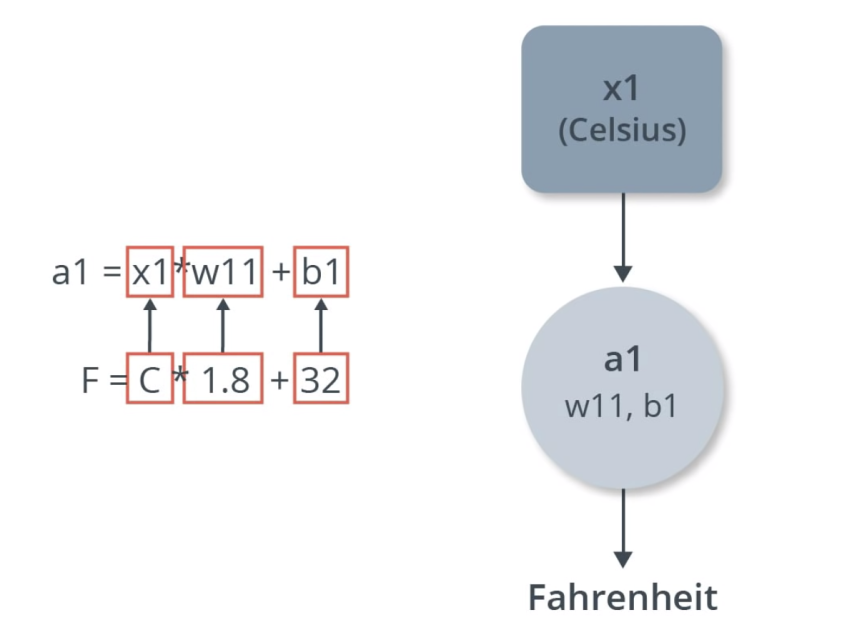
We’ll call the layer l0 and create it using tf.keras.layers.Dense with the following configuration:

• input_shape = [1]— This specifies that the input to this layer is a single value. That is, the shape is a one-dimensional array with one member. Since this is the first (and only) layer, that input shape is the input shape of the entire model. The single value is a floating point number, representing degrees Celsius (the feature).
• units = 1 — This specifies the number of neurons in the layer. The number of neurons defines how many internal variables the layer has to try to learn how to solve the problem. Since this is the final layer, it is also the size of the model’s output — a single float value representing degrees Fahrenheit (the labels). (In a multi-layered network, the size and shape of the layer would need to match the input_shape of the next layer.)

l0 = tf.keras.layers.Dense(units=1, input_shape=[1])  

Is this enough? As you will see later when checking the weights, the equation for weights and biases lines up with the actual Celsius to Fahrenheit equation.


Note that as the number of layers increase, so does the complexity of the equation. Below is a neural network with three layers:

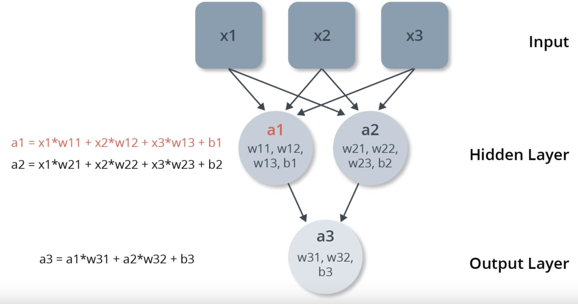
hidden = keras.layers.Dense(units = 2, input_shape = [3]) output = keras.layers.Dense(units = 1) model = tf.keras.Sequential([hidden, output])

• ASSEMBLE LAYERS INTO THE MODEL

Once the layers are defined, they need to be assembled into a model. A Sequential model takes a list of layers as an argument, specifying the calculation order from the input to the output.

model = tf.keras.Sequential([l0])

4. Compile the model, with loss and optimizer functions

Before training, the model has to be compiled. When compiled for training, the model is given a loss function and an optimizer function.

• Loss function — A way of measuring how far off predictions are from the desired outcome. The measured difference is called the “loss”.
• Optimizer function — A way of adjusting internal values in order to reduce the loss.

model.compile(loss = 'mean_squared_error',
optimizer = tf.keras.optimizers.Adam(0.1))

These calculate the loss at each point, and then adjust it. This is why it is called training.

During training, the optimizer function is used to calculate adjustments to the model’s internal variables. The goal is to adjust the internal variables until the model (which is really a math function) mirrors the actual equation for converting Celsius to Fahrenheit.

The loss function (mean squared error) and the optimizer (Adam) used here are standard for simple models like this one, but many others are available.

One part of the Optimizer you may need to think about when building your own models is the learning rate (0.1 in the code above). This is the step size taken when adjusting values in the model. If the value is too small, it will take too many iterations to train the model. Too large, and accuracy goes down. Finding a good value often involves some trial and error, but the range is usually within 0.001 (default), and 0.1

5. Train the model

During training, the model takes in Celsius values, performs a calculation using the current internal variables (called “weights”) and outputs values which are meant to be the Fahrenheit equivalent. Since the weights are initially set randomly, the output will not be close to the correct value. The difference between the actual output and the desired output is calculated using the loss function, and the optimizer function directs how the weights should be adjusted.

This cycle of calculate, compare, adjust is controlled by the fit method. The first argument is the inputs, the second argument is the desired outputs. The epochs argument specifies how many times this cycle should be run, and the verbose argument controls how much output the method produces. The cycle here is run 500 times and there are 7 Celsius/Fahrenheit pairs, so there are 3,500 examples total.

history = model.fit(celsius_q, fahrenheit_a, epochs = 500,
                    verbose = False)
print("Finished training the model")

6. Displaying training statistics

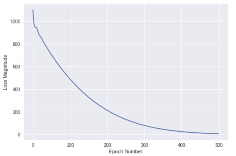
The fit method returns a history object. We can use this object to plot how the loss of our model goes down after each training epoch. A high loss means that the Fahrenheit degrees the model predicts is far from the corresponding value in fahrenheit_a.

We’ll use Matplotlib to visualize this (you could use another tool). As you can see, our model improves very quickly at first, and then has a steady, slow improvement until it is very near “perfect” towards the end.

import matplotlib.pyplot as plt
plt.xlabel('Epoch Number')
plt.ylabel("Loss Magnitude")
plt.plot(history.history['loss'])

7. Use the model to predict values

Now you have a model that has been trained to learn the relationship between celsius_q and fahrenheit_a. You can use the predict method to have it calculate the Fahrenheit degrees for a previously unknown Celsius degrees. Here let’s try 100C to F.

print(model.predict([100.0]))

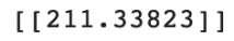
The correct answer is 100 × 1.8 + 32 = 212.

So far:

• We created a model with a Dense layer
• We trained it with 3,500 examples (7 pairs, over 500 epochs).
• Our model tuned the variables (weights) in the Dense layer until it was able to return the correct Fahrenheit value for any Celsius value. (Remember, 100 Celsius was not part of our training data.)

8. Looking at the layer weights

One can look at the internal variables of the Dense layer using .get_weights()

print("These are the layer variables: {}".format(l0.get_weights()))

Recall the real formula is: 𝑓 = 𝑐 × 1.8 + 32. So 1.8201642 is close to 1.8 and 29.321808 is pretty close to 32. Because we had a single input and output, the equation is 𝑦 = 𝑚𝑥 + 𝑏.

9. Experiment

Just for fun, what if we created more Dense layers with different units, which therefore also has more variables?

l0 = tf.keras.layers.Dense(units=4, input_shape=[1])
l1 = tf.keras.layers.Dense(units=4)
l2 = tf.keras.layers.Dense(units=1)
model = tf.keras.Sequential([l0, l1, l2])
model.compile(loss='mean_squared_error',
             optimizer=tf.keras.optimizers.Adam(0.1))
model.fit(celsius_q, fahrenheit_a, epochs=500, verbose=False)
print("Finished training the model")
print(model.predict([100.0]))
print("Model predicts that 100 degrees Celsius is:
      {} degrees Fahrenheit".format(model.predict([100.0])))
print("These are the l0 variables: {}".format(l0.get_weights()))
print("These are the l1 variables: {}".format(l1.get_weights()))
print("These are the l2 variables: {}".format(l2.get_weights()))

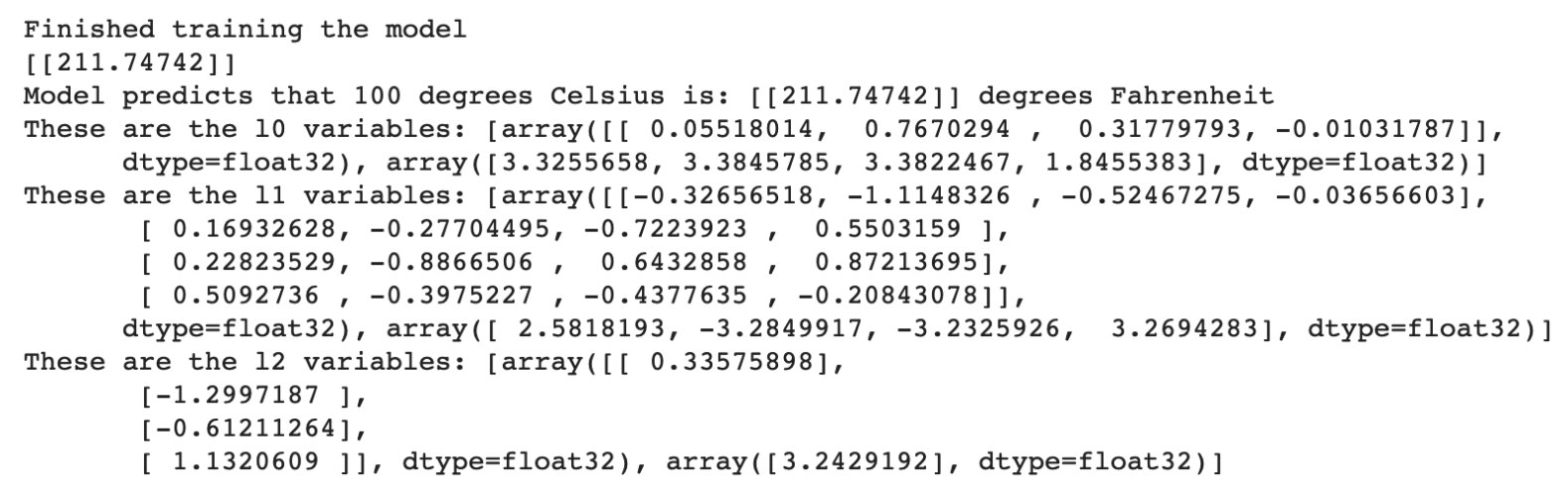
As you can see, this model is also able to predict the corresponding Fahrenheit value really well. But when you look at the variables (weights) in the l0, l1, and l2 layers, they are nothing even close to ~1.8 and ~32. The added complexity hides the “simple” form of the conversion equation.

Review and Terminology

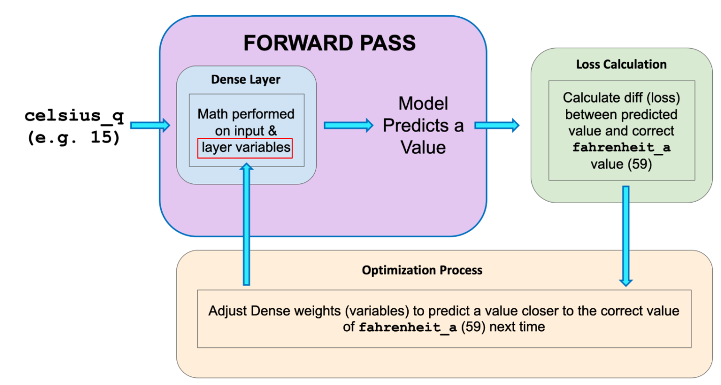
Figure 1. Forward Pass

The training process starts with a forward pass, where the input data is fed to the neural network. Then the model applies its internal math on the input and internal variables to predict an answer. In our example, the input was the degrees in Celsius, and the model predicted the corresponding degrees in Fahrenheit.

Once a value is predicted, the difference between that predicted value and the correct value is calculated. This difference is called the loss, and it’s a measure of how well the model performed the mapping task. The value of the loss is calculated using a loss function, which we specified with the loss parameter when calling model.compile().

After the loss is calculated, the internal variables (weights and biases) of all the layers of the neural network are adjusted, so as to minimize this loss — that is, to make the output value closer to the correct value.

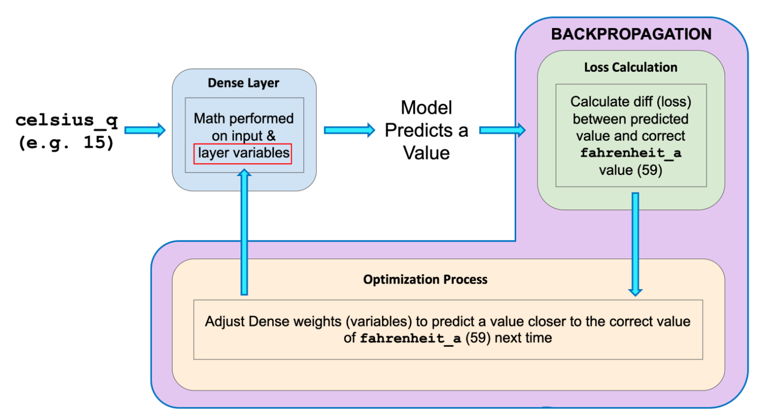
Figure 2. Back Propogation

This optimization process is called Gradient Descent. The specific algorithm used to calculate the new value of each internal variable is specified by the optimizer parameter when calling model.compile(...). In this example we used the Adam optimizer.

Terms:

• Feature: The input(s) to our model
• Examples: An input/output pair used for training
• Labels: The output of the model
• Layer: A collection of nodes connected together within a neural network.
• Model: The representation of your neural network
• Dense and Fully Connected (FC): Each node in one layer is connected to each node in the previous layer.
• Weights and biases: The internal variables of model
• Loss: The discrepancy between the desired output and the actual output
• MSE: Mean squared error, a type of loss function that counts a small number of large discrepancies as worse than a large number of small ones.
• Gradient Descent: An algorithm the internal variables a bit at a time to gradually reduce the loss function.
• Optimizer: A specific implementation of the gradient descent algorithm. (There are many algorithms for this. In this course we will only use the “Adam” Optimizer, which stands for ADAptive with Momentum. It is considered the best-practice optimizer.)
• Learning rate: The “step size” for loss improvement during gradient descent.
• Batch: The set of examples used during training of the neural network
• Epoch: A full pass over the entire training dataset
• Forward pass: The computation of output values from input
• Backward pass (back propagation): The calculation of internal variable adjustments according to the optimizer algorithm, starting from the output layer and working back through each layer to the input.